[O166] STS 51-L Right SRB

1.0. INTRODUCTION.

The STS 51-L Challenger disaster of 28 January 1986 was observed or measured by a number of sensors on the Eastern Test Range of ESMC. The STS 51-L Recovery Task Force has requested a report of all data evaluations pertinent to the Right Solid Rocket Booster (SRB), particularly those related to impact locations.

2.0. SUMMARY.

The right SRB elements appeared in the observations of the Ponce de Leon MIGOR and UCS-15 IFLOT optical trackers ETR Radars 1.17 and 0.14, and the FAA AN/FPS-66 Radar. Coverage by ETR radars and optical sites is depicted in Figure 1. Figure 2 is a map of sensors and impact locations, and Table 1 lists numerical values for impact locations and their estimated accuracies.

Impact Points R, RA, RC, and RD are confirmed elements of the right SRB. The altitude versus time profile for each of these objects is graphed in Figure 3. Impacts 2 through 7, representing targets detected by the FAA radar, are considered likely to be either right of left SRB elements, with the more Northerly impacts (2, 5, 6, 7) most likely being from the right SRB complex.

Report Section 3.0 which follows describes the right SRB data evaluations from ETR radars, ETR optical trackers, and the FAA radar. Section 4.0 describes the data processing for trajectory estimation and impact prediction. A reiteration of observations of the right SRB components is presented in summary fashion in Section 5.0.

3.0. DATA EVALUATION.

3.1. ETR Tracking Radars.

3.1.1. General.

Two impact locations related to the right SRB were derived from ETR tracking radar data. One of these objects, Object R, was estimated to be a major piece of the SRB aft segment.

3.1.2. Object R.

Following the structural breakup at T+73 seconds, Radar 1.17 shifted track to the right SRB which was positively identified by boresight video showing the anomalous plume. After Range Safety destruct at T+110 seconds, Radar 1.17 continued to track the largest SRB piece (predicted to be the Aft Segment and labeled Object R) until LOS near impact at T+286 seconds. Redundant track of the Right SRB by Radar 0.14 from T+89 to T+107 seconds was terminated by the Radar Controller, who directed Radar 0.14 to search for another object.

The altitude versus time profile for the Right SRB/Aft Segment is graphed in Figure 3. The altitude at destruct was about 102 K feet, and an apogee height of 123 K feet was reached at T+146 seconds.

The S/N recordings of Radars 1.17 and 0.14 during track of the intact SRB until T+110 seconds (Figure 4) showed peak Radar Cross Section (RCS) magnitudes up to 25 dBsm (decibels above a square meter), well below peak magnitudes observed later. These relatively small values were explained by the viewing geometry during the SRB's powered flight, which precluded broadside aspects and presented returns from the aft skirt and nozzle. During the track from T+110 to T+170 seconds, Radar 1.17 S/N recordings displayed periodic level variations typical of a tumbling object but did not show the specular returns which would be expected for broadside illumination of the SRB's cylindrical or conical surfaces.

The Radar 1.17 S/N recordings after T+170 seconds (Figure 5) displayed repetitive sequences which were typical of nearbroadside returns from both a cylindrical shape (symmetrical sidelobes) and a conical shape (asymmetrical sidelobes). The observed peak RCS magnitudes for each shape were compared with predicted values for various SRB segments (Tables 2), several of which were computed by Mr. M. Norton of RCA Data Processing. The peak RCS of the Object R cylinder was between 30.0 and 32.5 dBsm which, in relation to the SRB diameter of 12 feet, corresponded to a length between 7.0 and 9.4 feet. The peak RCS of the Object R conical portion was near 32.0 dBsm, which agreed closely with predicted values for the truncated cones of both the frustum (without nose cap) and aft skirt.

Conical plus cylindrical radar signature indicated that the tracked object was either the nose cone with attached forward skirt, or the aft skirt with a short section of SRB segment No. 1. Of these, the first was considered doubtful because of the absence of an orderly sidelobe structure which would be expected from the rather uniform surfaces; the second was believed to be more likely because the sidelobe irregularities could have resulted from surface components of the aft skirt or from the protruding nozzle.

Analysis of the ballistic characteristics of the metric trajectory (described later) predicted a weight of 73.5 K Ibs for the tracked object. This further substantiates that the tracked object was a major portion of the aft segment. Underwater photographs of the debris field emanating from the predicted impact point positively confirmed this identification.

3.1.3. Object RD.

Radar 0.14 tracked the right SRB from T+92 to T+106 seconds, and RTI (Range Time Intensity) displays processed at the DPDE facility from the recorded radar video output showed the presence of several separating pieces. Returns from these pieces ended when they left the antenna beam; i.e., at angular separations greater than 3 mils (approximately 550 feet) from the tracked object.

Figure 6a show returns from the SRB and seven separating pieces, displayed in a 45-km range window with fixed (constant range) window position. Figure 6b shows the same returns in an expanded 15-km window with the window start locked to the radar's range tracker. The "wiggles" in the Figure 6b traces are due to range tracker hunting as the separating pieces altered the centroid of the returns.

Metric range data were derived for Object RD, the separating piece visible until T+96 seconds in Figures 6a and 6b, by applying RTI range differentials to Radar 0.14 range-tracker data. The derived range measurements, displayed graphically in Figure 7, were utilized in a NITE BET computer run to estimate the impact location for Object RD.

Signal amplitude data for signature analysis were obtained by a playback track at the DPDE for the time span of T+93.6 to T+95.8 seconds. Figures 8a and 8b show signal amplitudes for the SRB and Object RD, respectively, from playback tracks. The signature of Object RD reveals a sequence of features (marked by arrows in Figure 8b) repeating at 0.8 second intervals, which suggests tumble or spin. These broad features may have originated from a small, fairly flat surface.

The peak RCS of Object RD was only .06 m² ( -12.6 dBsm) and average RCS was about .005 m² (-23 dBsm). The values contrast with SRB values up to 5,000 m² (37 dBsm) during the same time span.

Unfortunately Radar 0.14 is the only Mainland ETR radar with receiver video recording capability. Consequently similar data on small pieces expelled from the SRB cannot be obtained from the other radar tracks.

3.2. ETR Optical Trackers.

3.2.1. General.

Optical tracking coverage, other than radar boresight video, of the right SRB was from the Ponce de Leon (PDL) MIGOR and UCS-15 IFLOT, was located as shown in Figure 1.

3.2.2 Discussion.

All of the optical trackers, with exception of UCS- 10 MIGOR and Melbourne Beach ROTI, were tasked to track the Orbiter/ET until LOV. UCS-10 was to track the north (right) SRB after separation and Melbourne Beach ROTI the south (left) SRB.

After the mishap at T+73 seconds, most camera operators searched for the Orbiter, tracking only briefly on pieces of debris.

[O167] Occasionally during their search, SRB's passed through the field of view. Where a track on an SRB did occur, it was only for a short period of time, not more than 10 seconds. Long periods of track were devoted to the parachutes.

Radar 1.17 and the PDL MIGOR tracked a common target to impact as confirmed by a comparison of the radar tracking data, transformed to the MIGOR Site, with the MIGOR data. Data throughout the track agreed to -0.1 degree.

The right SRB could be readily identified because of its double plume. From the MIGOR tracking video, before command destruct, the double plume was prominently visible and provided the proof that the MIGOR was tracking the right SRB and therefore the 1.17 radar also tracked the right SRB. Film data were not available from the PDL MIGOR because of film breakage.

That part of the right SRB tracked by Radar 1.17 and PDL MIGOR was determined to be the aft section from radar signature data, weight estimates from the NITE computer program and underwater pictures.

The PDL video, at command destruct, showed that the SRB separated into a number of pieces. Three pieces, of near equal luminosity, remained in the field of view for several seconds. Two of the pieces, which have been designated Objects RA and RB, were continuously visible while in the field of view; but the third piece, Object RC, flashed on and off. Trajectories of these pieces, as seen in the video plane relative to the tracked aft section, are shown in Figure 9.

Another piece, flashing at approximately 2 flashes per second, appeared suddenly and remained in the field of view for nearly twenty seconds. It is shown in figure 10. The object's origin was tentatively identified as the aft segment of the right SRB but this could not be positively confirmed since it is visible only intermittently. Subsequent video image enhancement identified 2 more positions tieing the object back to the aft segment.

A review of available data, both film and video tapes, revealed that the UCS-15 IFLOT was the only other instrument tracking the right SRB at the time of destruct command. Figures 11 through 14 are UCS-15 photographs at I second intervals beginning at T+111.026 seconds. It can readily be seen that a large number of pieces came from the SRB. The four bright objects remaining, see Figure 14, have been correlated with the bright objects seen from PDL. Knowing the position of the aft section (brightest object in the photo) pointing angles could be computed to each of the objects from the measured in-plane offsets. This was accomplished for each picture frame (30 per second) while the objects were in the field of view. These data, in conjunction with the PDL data, were the basis for triangulations and trajectory generations. It is to be noted that the UCS-15 IFLOT is only an engineering sequential camera, i.e., having only timing recorded on the film and no mount orientation data. The mount orientation can only be determined if a target whose spatial coordinates are known is visible in the field of view. Fortunately, since the aft section was tracked by radar, its spatial position was known and orientation angles could be computed.

There are several smoking objects seen in the photos, one of which also seemed to be visible in the PDL video. Work is underway to read the offsets of all visible objects relative to the aft section on both the PDL video and UCS-15 film.

The video was read with a TV tracker at 10 samples per second. Each sample was read during still framing of the video. Objects which can just be seen dynamically (continous projection) fade into the background when viewed statically (single frame projection); thus, not all of the visible objects can be read with the present equipment. Possibly with the use of more sophisticated equipment, computer enhancements, etc., additional data might be forthcoming.

The shock wave from the Range Safety command destruct explosion was visible on the 16mm film from Camera E-705 installed on the UCS-15 mount. Measurements of the shock wave width versus time fit an inverted power curve as shown in Figure 15.

Regression to zero width gives the explosion at time T+ 110.275 seconds. The propagation speed of the shock wave was on the order of 1000 m/s during the first few hundredths of a second with the expansion slowing to essentially zero within . I second.

3.3. AN/FPS-66 Radar.

3.3.1. General.

The AN/FPS-66 radar is located at the southern extremity of Patrick AFB, on the west side of Route A1A, with a very favorable view for targets over the ocean. It scans at 5 revs/minute, detecting significant targets below 70,000 feet. The beam is 1.3° wide and the PRF is 360/second, so adequate targets yield about 15 successive returns on each beam passage. The radar is operated by FAA and the data are processed for map presentation by the FAA's Jacksonville ARTC Center of Hilliard, Florida. The maps of target detections were examined for corroboration of impact "R" (well-established by NITE processing of Radar 1.17), and then 6 more target impacts were found which appeared to be credible.

It must be remembered that no elevation or height data was measured, so slant range-to-ground range conversions could not be made. In the FAA data format, map granularity of one-third mile limited the plotting precision, but latitude/longitude values were also listed for improved accuracy.

3.3.2. Discussion.

The target impacting at location R was well-documented from Radar 1.17 measurements of trajectory and radar cross section, and boresight television recordings. This same target was first detected by the FPS-66 at T+ 221 seconds, for which the altitude was known to be 50 K feet.

The target was observed at successive 12-second intervals through the known time of impact. These observations were classified as "long run length primary," indicating a well-confirmed or strong target return. After the known impact time, the FPS-66 continued to register hits downrange of the impact location which were of lesser confidence or "short run length primary" classification. These reflections were real, but must have been very light following debris or ashes that were not targets of substance.

The behavior just described for target manifestations in FPS-66 data were considered in the selection of significant targets from the remainder of the mapped detections. Re-entry appearance was assumed at about 50 to 70 K feet, and impact was reasoned to be about 5 observations (I minute) later, with large targets meeting the criterion of"long run length primary."

The map regions under examination were those appropriate for an SRB target. (Since the SRB's had thrust for 38 seconds after the Orbiter structural breakup, the area of interest was further east than Orbiter/ET debris.) In this region the target density was not great, and discrete target traces could be more readily discerned.

The six target impacts shown in Table 1 were selected from the FAA data because each appeared to qualify by the "reasonableness" criteria applicable to known target "R".

However, except for proximity to "R", the six cannot be qualified as definitely portions of the right SRB, rather than the left SRB. Corroborative data from other trackers do not exist for these targets.

The data to Table 1 for targets 2 through 6 have been estimated somewhat coarsely regarding time of impact and the impact uncertainty ellipse. Since radar observations occurred at 12-second intervals with no altitude information, confidence in time values is about +/- 12 seconds. The error ellipse shape and size reflects the observed dispersion of points on the original mapped data.

The great value of the FPS-66 radar has been its overall coverage of the accident scene, permitting some hits on all significant targets. The difficulty in using the data has been in the discrimination between significant targets and the multitude of small reflectors.

Feed back from the sonar search activities indicated returns at all but one of the impacts predicted from the FAA radar data. Due to the initial success and usefulness of these predictions, the [O168] FAA radar data was thoroughly reanalyzed to see if additional probable tracks and impacts could be extracted. Eleven additional impact locations (having confidence estimates similar to the original figure 7) were extracted and are listed in Table 4.

The FAA data have been forwarded to specialists in the National Transportation Safety Boards in Washington, DC for further analysis for the Recovery Task Force.

4.1. General.

Vehicle performance and impact prediction are normally routine and accurate computations are based upon extended tracking data from several radars or optical instruments. Only a very few of the STS 51-L pieces had long track spans or multiple instrument coverage. Impacts for those pieces were readily predicted with high accuracy. The challenge, however, was to provide useful impact accuracies for many objects which were observed for only a few seconds or did not have full "metric" data. The metric optical instruments on the range provided azimuth, elevation (and time) data on the tracked object. Position is computed by a triangulation process. Tracking offsets can be read post-test and used to correct the pedestal data in order improve trajectory accuracy. Accuracy can be further improved by using data from additional (redundant) trackers. For short periods of time after the initial structural breakup and after booster destruct, numerous non-tracked objects were visible in the film and TV recordings from the various optical sensors (metric optics, engineering sequential optics, and radar boresight video). Azimuth and elevation data from these objects can be computed by reading the angular offsets from the tracked object and suitably combining them with the pedestal metric data. If the object can be positively identified in data from two different camera sites, a triangulation can be performed to compute trajectory position. In the case of engineering sequential cameras only time data is recorded on the film and thus there is no azimuth or elevation data directly available for the optical axis. However, if there is some object visible in the frame for which full position data is available from any other source, the camera orientation can be computed and the data can be handled essentially the same as for the metric optics. In cases where there is only single camera coverage and triangulation is not possible a ballistic constraint can be used to estimate the trajectory. This approach becomes more accurate as the tracking span length increases.

The NITE program was used to perform these complex trajectory computations. It fits a set of redundant measurements best in a least-squares sense. The program permits user-definition of the gravitational and drag forces and the appropriate wind conditions. The trajectory fit also contrains the measurements to fit the equations of motion. The fitted data produced estimates of the drag parameter and the initial conditions of a position/velocity vector; then the equations of motion were numerically integrated to produce an impact point.

A measure of the accuracy of the impact location is provided by the parameters of the 95 % confidence ellipse. The major and minor axes along with the azimuth of the major axis is given with the impact locations in Table 1.

Figure 2 illustrates the locations of the launch pad, instrumentation sites, and impact points. For Object R, the ground trace is provided from launch to impact.

Program NITE "N-Interval Trajectory Estimation," No.615 has been used at ESMC and WSMC for many years, and is a well known reference.

4.2. Object R.

As stated in an earlier section, Radar 1.17 tracked the aft section to impact. However, the 1.17 RAE data were processed by computer program NITE to provide a "Best Estimate of Trajectory" including the impact location. This added confidence to the impact point already obtained from computer program RAPP. When meteorological data (including atmospheric density, wind speed, and direction) were used as part of the dynamics model, the NITE solution differed from the already obtained impact point by 59 feet. The NITE run also indicated the importance of using the wind data in NITE solutions involving other pieces.

Specifically, for the aft section, the impact point computed using wind data differed from the impact point computed without winds by approximately one-half mile. Figures 16 and 17 illustrate the wind speed and direction that were used.

Data from Radar 1.17 provided an initial estimate of the position and velocity vector. Marshall Space Flight Center (MSFC) provided information on the drag parameters for both a Tail-First descent and a Tumbling descent; see Figure 18. The NITE run using the drag for a Tail-First descent was judged to be slightly better than the run using tumbling descent drag for Plots of velocity and acceleration versus time are provided in Figures 19-26.

4.3. Objects RA, RB, and RC.

The impact locations for these three pieces of the right SRB were computed using measurements from Ponce de Leon video recording and UCS-15 70mm and 16mm films. These pieces are referred to as RA, RB, and RC. Data time spans and data frequency are listed in Table 3.

For each of the three pieces the same procedure was used to process the data in order to obtain an estimated impact location.

Computer program TCAR (No. 017: Tracking Camera Automatic Reduction) was used (1) to transform the video and film readings to azimuth and elevation angles, and (2) to compute an initial estimate of the position vector at times when triangulation was possible. An estimate of the velocity vector at the beginning of a data span was computed manually by using difference techniques.

The azimuth and elevation data along with the position and velocity vector were then input into computer program NITE to obtain an impact point.

4.4. Object RD.

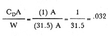
A small amount of range data was obtained from RTI (Range Time Intensity) recordings. This range data along with an initial position and velocity vector for 1.17 radar data were processed in the NITE program to obtain an impact point. The drag parameter used was obtained from MSFC data, assuming this piece was a tumbling SRB segment.

Specifically, using C_D = 1.0 and W= 31.5, A gives the drag parameter,

Notice that with this model the "ballistic" coefficient is independent of the size of the piece. The coefficient however, is highly dependent upon the assumption for C_D.

4.5 Object Weights.

4.5.1 Estimates of Object Weight.

Computer program NITE can solve for the "ballistic coefficient" product-quotient where

where

C_D = Coefficient of drag

A = Surface Area

W = Weight

If one assumes that C_D and A are known, then W can be computed using the formula

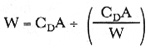
Using C_D and the reference area A obtained from MSFC estimated weights are

Estimates of empty weight for the SRB segments as provide, by MSFC are:

Note that Object R appears to be a major portion of the Aft Segment. Other objects (RA, RB, RC) appear to be less than one-half of the forward and center segments.

Early underwater photographs indicated that the booster pieces had a layer of unburned fuel attached. Unburned fuel would increase the object weight without significantly modifying the drag coefficient or reference area. Both TV and film indicated that fuel was still glowing after destruct. This additional and possibly changing weight could have an important effect on the ballistic trajectory and several models were analyzed to determine its significance in impact locations. Although the fuel might increase the initial weight by 30%, it was expected to be largely burned off before the objects entered the denser atmosphere where the ballistic coefficient has greater effect. An impact uncertainty of approximately 0.7 nm could be expected in impact location due to this effect. The uncertainty in impact time is considerably greater but has little importance to recovery operations.

4.5.2. Comments on Weight Estimates Using Short Spans of Data

To investigate how well a weight can be determined from relatively short spans of data, several computer runs were made using short spans of Radar 1.17 data. Using data from 115125 seconds at 10 pps resulted in a weight estimate of 75,400 Ibs for the aft section.

Using data from 115- 120 seconds at 10 pps resulted in a weight estimate of 91,600 Ibs for the aft section.

These estimates are to be compared to the estimate of 73,500 Ibs obtained by using data from the total tracking span of 115-270 seconds.

4.5.3. The Effect of Drag Parameter on Impact Location

If C_D and A are considered known, then the unknown variable in C_DA/W is, of course, the weight W. Inaccurate estimates of W result in inaccurate estimates of C_DA/W. When an inaccurate estimate of C_DA/W is used in the computation of an impact point, that impact point is in error. A measure of the effect of C_DA/W will now be given.

Using the initial position and velocity associated with Object RA, trajectories were generated using different weights. Impact points were obtained using weights of 21,000 Ibs, 10,500 Ibs and 5,000 Ibs. The impact location associated with 10,500 Ibs was 3.3 nm from the impact location associated with the 21,000 lb weight. The impact location associated with using a weight of 5,000 Ibs was 6.2 nm from the impact location obtained using a weight of 21,000 Ibs.

5.0. Condensed Chronology of Right SRB Observations.

Following the structural break-up at T+ 73 seconds, the right Solid Rocket Booster continued under thrust for approximately 37 seconds. It was tracked continuously by Radar 1.17 and Ponce de Leon MIGOR. Radar 0.14 and the UCS-15 IFLOT tracked briefly as shown in Figure 1.

Analysis of the PDL MIGOR video tape shows the SB to be rolling clockwise viewed from aft approximately once every 10 seconds during the powered flight period. Possibly this period decreased by about 1.5 seconds during the 37 seconds of powered flight indicating an angular acceleration about the longitudinal axis.

From T+93.6 to T+95.8 seconds Radar 0.14 detected a number of small objects separating from the main target (Figures 6 and 7.). None of these objects were visible to the optics sites or on the radar boresight video tape. Enough data could be extracted to permit a trajectory estimate to be made for one of these objects (designated RD on Figure 2). Impact was at approximately T+398 seconds, and the separation speed relative to the main SRB body was on the order of 123 meters/second.

At T + 110.3 seconds Range Safety issued a command destruct to the Solid Rocket Booster. The shock wave from the destruct explosion of the right SRB was visible on the UCS-15 E-705 16mm camera (Figure 15), permitting a computed estimate of the explosion at time T+ 110.275 seconds. The propagation speed of the shock wave was on the order of 1,000 m/s during the first few hundredths of a second with the expansion slowing to essentially zero within 0.1 second.

Following the command destruct, the SRB separated into a number of fragments as shown by the photos Figures 11 through 14. Optical resolution was not sufficient to permit the identification of these fragments. Radar I .17 and PDL MIGOR continued to track a large piece later identified as part of the aft segment and skirt. A number of smoke trails, possibly two dozen small (pinpoint) glowing objects, and four bright glowing objects could be seen on the UCS-15 IFLOT 70mm film. The four bright glowing objects and possibly three smoke trails were also seen on the PDL MIGOR video tape. The radar boresight video tape showed no visible object after the command destruct.

Because the smoke trails are at the limit of the PDL MIGOR video resolution, first priority was given to the three bright glowing objects not tracked by Radar 1.17. Triangulation on these Objects (RA, RB, and RC) was possible for periods of 4 to 6 seconds, and impact trajectories have been generated. Table 1 lists the impact times and positions and Figure 2 is a map showing the ground traces of the tracked (solid) and projected (dotted) trajectories. Separation speeds relative to the booster aft segment ranged from 45 m/s to 120 m/s.

From T+115 to T+141 seconds, and object flashing twice per second was in the PDL MIGOR field of view (Figure 10). It appears after image enhancement to originate from the aft segment of the right SRB.

The FAA radar observations cannot be positively associated with the right or the left SRB. The six initial impact estimates are shown in Table 1 and the next 11 estimates are listed in Table 4.

[O170] TABLE 1: IMPACT ESTIMATES AND UNCERTAINTY ELLIPSE.

NOTES: The FAA radar target identified by #1 was the same as target R.

[O171] TABLE 2: CALCULATED C-BAND RCS.

* Aft Segment

[O172] TABLE 3: DATA INPUT TO NITE PROGRAM.

---

[O173]

Figure 1. ETR CAMERA AND RADAR COVERAGE OF RIGHT SRB.

---

---

[O174]

Figure 2. RIGHT SRB AND FAA RADAR IMPACTS.

---

---

[O175]

Figure 3. OBJECT ALTITUDE VERSUS TIME.

---

---

[O176]

Figure 4. RADAR 1.17 and O.14 PDV RECORDINGS DURING SRB TRACK.

---

---

[O177]

Figure 5. RADAR 1.17 PDV RECORDING.

---

---

[O178]

Figure 6. a) Range/Intensity vs. Time, Fixed Window. B) Range/Intensity vs. Time, Moving Window.

---

---

[O179]

Figure 7. RADAR 0.14 RANGE DATA.

---

---

[O180]

Figure 8. RADAR 0.14 VIDEO RECORDINGS AT DPDE. a) Signal Amplitude vs. Time, Track of SRB.

b) Signal Amplitude vs. Time, Playback Track of Separating Target.

---

---

[O181]

Figure 9. PDL MIGOR VIDEO OFFSETS.

---

---

[O182]

Figure 10. PDL MIGOR VIDEO OFFSETS FOR FLASHER.

---

---

[O183]

Figure 11. Right SRB T+111.026 Seconds. Instrument: UCS-15 IFLOT.

Figure 12. Right SRB T+112.026 Seconds. Instrument: UCS-15 IFLOT.

---

---

[O184]

Figure 13. Right SRB T+113.026 Seconds. Instrument: UCS-15 IFLOT.

Figure 14. Right SRB T+114.026 Seconds. Instrument: UCS-15 IFLOT.

---

---

[O185]

Figure 15. RANGE-DESTRUCT SHOCKWAVE RADIUS VS TIME.

---

---

[O186]

Figure 16. RAWINSONDE ASCENT NO 147.

---

---

[O187]

Figure 17. RAWINSONDE ASCENT NO 147.

---

---

[O188]

Figure 18. SRB AFT SEGMENT DRAG COEFFICIENT (Obtained from MSFC)

---

---

[O189]

Figure 19. [blank page?]

---

---

[O190]

Figure 20. OBJECT R VELOCITY DATA.

---

---

[O191]

Figure 21. OBJECT R VELOCITY DATA.

---

---

[O192]

Figure 22. OBJECT R VELOCITY DATA.

---

---

[O193]

Figure 23. OBJECT R VELOCITY DATA.

---

---

[O194]

Figure 24. OBJECT R ACCELERATION DATA.

---

---

[O195]

Figure 25. OBJECT R ACCELERATION DATA.

---

---

[O196]

Figure 26. OBJECT R ACCELERATION DATA.

---

[O197] TABLE 4: ADDITIONAL IMPACT ESTIMATES FROM THE FAA AN/FPS-66 RADAR.

Uncertainty ellipse orientations = 120°

Semi-major Axes (nm) = 0.75

Semi-minor Axes (nm = 0.25

[O198] GLOSSARY.

ESMC Range Instrumentation.

A.1. General.

Instrumentation utilized by ESMC, which includes resources of other agencies, is summarized in Figure A-1.

A.2. Tracking Radars.

The C-Band radars listed in Table A-l are used for Range Safety purposes and for provided metric data to the Range User. All ESMC tracking radars are azimuth-elevation-range sensors which do not have provisions for range-doppler measurements. Each radar is equipped with a boresight TV camera and recorder to assist with calibration and mission support.

The FPQ-13, FPQ-14, and FPQ-15 radars are "On-Axis" types which utilize computer processing of receiver signals and tracking algorithms in order to enhance precision. In addition to metric data, On-Axis radars compute and record signature data

(Signal/Noise and RCS) at full PRF rate of 160 Hertz. Radar 91.14 is equipped for on-site precording of receiver video, and Radar 0.14 receiver video is recorded at the Patrick Tech Lab DPDE facility.

The mobile MCBRs utilize an equipment van and a pedestal trailer. These radars can be positioned for most effective mission support in the CCAFS/KSC area or dispatched to remote locations such as Jupiter, Florida.

A.3. Optics.

The optical instruments listed in Table A-2 collect metric data, comprised of azimuth and elevation measurements, and engineering sequential data which document mission events. Data are recorded on photographic film or video tape.

A.4. Surveys.

The geodetic location of radar and optical sites are listed in Tables A-3 and A-4, respectively.

[O200] TABLE A-1: ESMC C-BAND TRACKING RADARS.

[O201] TABLE A-2: ESMC OPTICAL INSTRUMENTS.

NOTES:

1) All instruments except IFLOT are equipped with azimuth and elevation encoders.

2) The tracking scope (1 meter focal length) of the Ponce MIGOR is equipped with TV camera and recorder.

3) Located northeast of UCS-12 site.

4) Sites are listed by latitude, north to south

[O202] TABLE A-3: GEODETIC COORDINATES FOR ESMC C-BAND RADARS.

TABLE A-4: GEODETIC COORDINATES FOR ESMC OPTICAL SITES.

---

[O203]

Figure A-1. ESMC RANGE INSTRUMENTATION FACILITIES

---